Library: September 2011

Sunday, 18 September 2011

What does it take to become a hacker?

What does it take to become a hacker?

Becoming a great hacker isn’t easy and it doesn’t happen quickly. Being
creative helps a lot. There is more than one way a problem can be solved, and as
a hacker you encounter many problems. The more creative you are the bigger
chance you have of hacking a system without being detected. Another huge
quality you must have is the will to learn because without it, you will get
nowhere. Remember, Knowledge is power. Patience is also a must because many
topics can be difficult to grasp and only over time will you master them.

Hacker Hierarchy

Hacker Hierarchy

Script kiddies – These are the wannabe hackers. They are looked down upon in
the hacker community because they are the people that make hackers look bad.
Script kiddies usually have no hacking skills and use the tools developed by other
hackers without any knowledge of what’s happening behind the scenes.
Intermediate hackers – These people usually know about computers, networks,
and have enough programming knowledge to understand relatively what a script
might do, but like the script kiddies they use pre-developed well-known exploits (-
a piece of code that takes advantage of a bug or vulnerability in a piece of software that allows
you to take control of a computer system) to carry out attacks
Elite Hackers – These are the skilled hackers. They are the ones that write the
many hacker tools and exploits out there. They can break into systems and hide
their tracks or make it look like someone else did it. You should strive to
eventually reach this level.

What is a hacker?

What is a hacker?

A hacker is someone who likes to tinker with electronics or computer
systems. Hackers like to explore and learn how computer systems work, finding
ways to make them do what they do better, or do things they weren’t intended to
do. There are two types of hackers:

White Hat – These are considered the good guys. White hat hackers don’t use
their skills for illegal purposes. They usually become Computer Security experts
and help protect people from the Black Hats.

Black Hat – These are considered the bad guys. Black hat hackers usually use their
skills maliciously for personal gain. They are the people that hack banks, steal
credit cards, and deface websites.

These two terms came from the old western movies where the good guys wore
white hats and the bad guys wore black hats.
Now if you’re thinking, “Oh boy! Being a black hat sounds awesome!”, Then I have
a question for you. Does it sound cool to live in a cell the size of your bathroom
and be someone’s butt buddy for many years? That’s what I thought.

Abell, George O. (1927–1983) American Astronomer

Determining the nth occurrence of a day of the week in a month

You may need a formula to determine the date for a particular occurrence of a weekday. For
example, suppose your company payday falls on the second Friday of each month, and you need
to determine the paydays for each month of the year. The following formula makes this type of
calculation:

=DATE(A1,A2,1)+A3-WEEKDAY(DATE(A1,A2,1))+
(A4-(A3>=WEEKDAY(DATE(A1,A2,1))))*7

The formula in this section assumes that

      Cell A1 contains a year.

      Cell A2 contains a month.

      Cell A3 contains a day number (1 for Sunday, 2 for Monday, and so on).

      Cell A4 contains the occurrence number (for example, 2 to select the second occurrence
        of the weekday specified in cell A3).

If you use this formula to determine the date of the second Friday in November 2010, it returns
November 12, 2010.

             If the value in cell A4 exceeds the number of the specified day in the month, the for-
             mula returns a date from a subsequent month. For example, if you attempt to deter-
             mine the date of the fifth Friday in November, 2010 (there is no such date), the formula
             returns the first Friday in December.

Determining the day of the week

Determining the day of the week

The WEEKDAY function accepts a date argument and returns an integer between 1 and 7 that
corresponds to the day of the week. The following formula, for example, returns 7 because the
first day of the year 2011 falls on a Saturday:

=WEEKDAY(DATE(2011,1,1))

The WEEKDAY function uses an optional second argument that specifies the day numbering sys-
tem for the result. If you specify 2 as the second argument, the function returns 1 for Monday, 2
for Tuesday, and so on. If you specify 3 as the second argument, the function returns 0 for
Monday, 1 for Tuesday, and so on.

             You can also determine the day of the week for a cell that contains a date by applying a
              custom number format. A cell that uses the following custom number format displays
              the day of the week, spelled out:

                 dddd

Determining the date of the most recent Sunday

You can use the following formula to return the date for the previous Sunday. If the current day is
a Sunday, the formula returns the current date. (You will need to format the cell to display as a
date.)

=TODAY()-MOD(TODAY()-1,7)

To modify this formula to find the date of a day other than Sunday, change the 1 to a different
number between 2 (for Monday) and 7 (for Saturday).

Determining the first day of the week after a date

This next formula returns the specified day of the week that occurs after a particular date. For
example, use this formula to determine the date of the first Monday after June 1, 2010. The for-
mula assumes that cell A1 contains a date and that cell A2 contains a number between 1 and 7 (1
for Sunday, 2 for Monday, and so on).

=A1+A2-WEEKDAY(A1)+(A2<WEEKDAY(A1))*7

If cell A1 contains June 1, 2010 (a Tuesday), and cell A2 contains 7 (for Saturday), the formula
returns June 5, 2010. This is the first Saturday after June 1, 2010.

Where’s the DATEDIF function?

   In several places throughout this chapter, I refer to the DATEDIF function. You may notice that
   this function does not appear in the Insert Function dialog box, is not listed in the Date & Time
   drop-down list, and does not appear in the Formula AutoComplete list. Therefore, to use this
   function, you must always enter it manually.

   The DATEDIF function has its origins in Lotus 1-2-3, and apparently Excel provides it for compat-
   ibility purposes. For some reason, Microsoft wants to keep this function a secret. You won’t even
   find the DATEDIF function in the Help files, although it’s available in all Excel versions. Strangely,
   DATEDIF made an appearance in the Excel 2000 Help files but hasn’t been seen since.

   DATEDIF is a handy function that calculates the number of days, months, or years between two
   dates. The function takes three arguments: start_date, end_date, and a code that represents the
   time unit of interest. Here’s an example of a formula that uses the DATEDIF function (it assumes
   cells A1 and A2 contain a date). The formula returns the number of complete years between
   those two dates.

   =DATEDIF(A1,A2,”y”)

   The following table displays valid codes for the third argument. You must enclose the codes in
   quotation marks.

    Unit Code      Returns

    “y”            The number of complete years in the period.

    “m”            The number of complete months in the period.

    “d”            The number of days in the period.

    “md”           The difference between the days in start_date and end_date. The months and years
                   of the dates are ignored.

    “ym”           The difference between the months in start_date and end_date. The days and years
                   of the dates are ignored.

    “yd”           The difference between the days of start_date and end_date. The years of the dates
                   are ignored.

   The start_date argument must be earlier than the end_date argument, or the function returns an
   error.

Here’s a similar formula that returns the day of the year for the current date:

=TODAY()-DATE(YEAR(TODAY()),1,0)
=DATE(YEAR(A1),12,31)-A1

When you enter either of these formulas, Excel applies date formatting to the cell. You need to
apply a non-date number format to view the result as a number.

To convert a particular day of the year (for example, the 90th day of the year) to an actual date
in a specified year, use the formula that follows. This formula assumes that the year is stored in
cell A1 and that the day of the year is stored in cell B1.

=DATE(A1,1,B1)

Calculating a person’s age

A person’s age indicates the number of full years that the person has been alive. The formula in
the previous section (for calculating the number of years between two dates) won’t calculate this
value correctly. You can use two other formulas, however, to calculate a person’s age.

The following formula returns the age of the person whose date of birth you enter into cell A1.
This formula uses the YEARFRAC function:

=INT(YEARFRAC(TODAY(),A1,1))

The following formula uses the DATEDIF function to calculate an age. (See the sidebar, “Where’s
the DATEDIF function?”)

=DATEDIF(A1,TODAY(),”y”)

Determining the day of the year

January 1 is the first day of the year, and December 31 is the last day. But what about all of those
days in between? The following formula returns the day of the year for a date stored in cell A1:

=A1-DATE(YEAR(A1),1,0)

The day argument supplied is zero, calling for the “0th” day of the first month. The DATE func-
tion interprets this as the day before the first day, or December 31 of the previous year in this
example. Similarly, negative numbers can be supplied for the day argument.

Calculating the number of years between two dates

Calculating the number of years between two dates

The following formula calculates the number of years between two dates. This formula assumes
that cells A1 and B1 both contain dates:

=YEAR(A1)-YEAR(B1)

This formula uses the YEAR function to extract the year from each date and then subtracts one
year from the other. If cell B1 contains a more recent date than the date in cell A1, then the result
is negative.
You can also use the YEARFRAC function to calculate the number of years between two dates.
This function returns the number of years, including partial years. For example

=YEARFRAC(A1,B1,1)

Because the YEARFRAC function is often used for financial applications, it uses an optional third
argument that represents the “basis” for the year (for example, a 360-day year). A third argu-
ment of 1 indicates an actual year.

Converting a non-date string to a date

Converting a non-date string to a date

You may import data that contains dates coded as text strings. For example, the following text
represents August 21, 2010 (a four-digit year followed by a two-digit month, followed by a two-
digit day):

20100821

To convert this string to an actual date, you can use a formula such as this one, which assumes
the coded date is in cell A1:

=DATE(LEFT(A1,4),MID(A1,5,2),RIGHT(A1,2))

Calculating the number of years between two dates

Calculating the number of years between two dates

The following formula calculates the number of years between two dates. This formula assumes
that cells A1 and B1 both contain dates:

=YEAR(A1)-YEAR(B1)

This formula uses the YEAR function to extract the year from each date and then subtracts one
year from the other. If cell B1 contains a more recent date than the date in cell A1, then the result
is negative.

Displaying any date

Displaying any date

As explained earlier in this chapter, you can easily enter a date into a cell by simply typing it,
using any of the date formats that Excel recognizes. You can also create a date by using the
DATE function, which takes three arguments: the year, the month, and the day. The following for-
mula, for example, returns a date comprising the year in cell A1, the month in cell B1, and the day
in cell C1:

=DATE(A1,B1,C1)

              The DATE function accepts invalid arguments and adjusts the result accordingly. For
              example, this next formula uses 13 as the month argument, and returns January 1, 2010.
              The month argument is automatically translated as month 1 of the following year.

                  =DATE(2009,13,1)

Often, you’ll use the DATE function with other functions as arguments. For example, the formula
that follows uses the YEAR and TODAY functions to return the date for Independence Day (July
4th) of the current year:

=DATE(YEAR(TODAY()),7,4)

The DATEVALUE function converts a text string that looks like a date into a date serial number.
The following formula returns 40412, the date serial number for August 22, 2010:

=DATEVALUE(“8/22/2010”)

Date-Related Functions

Date-Related Functions

Excel has quite a few functions that work with dates. They are all listed under the Date & Time
drop-down list in the Formulas➜Function Library group.

Table 6-4 summarizes the date-related functions available in Excel.

Table 6-4: Date-Related Functions

Function                      Description

DATE                          Returns the serial number of a date given the year, month, and day

DATEDIF                       Calculates the number of days, months, or years between two dates

DATEVALUE                     Converts a date in the form of text to an actual date

DAY                           Returns the day of the month for a given date

DAYS360                       Calculates the number of days between two dates based on a 360-day year

EDATE*                        Returns the date that represents the indicated number of months before or
                              after the start date

EOMONTH*                      Returns the date of the last day of the month before or after a specified num-
                               ber of months

MONTH                         Returns the month for a given date

NETWORKDAYS*                  Returns the number of whole work days between two dates

NETWORKDAYS.INTL**            An international version of the NETWORKDAYS function

NOW                           Returns the current date and time

TODAY                         Returns today’s date

WEEKDAY                       Returns the day of the week (expressed as a number) for a date

WEEKNUM*                      Returns the week number of the year for a date

WORKDAY*                      Returns the date before or after a specified number of workdays

WORKDAY.INTL**               An international version of the WORKDAY function

YEAR                          Returns the year for a given date

YEARFRAC*                     Returns the year fraction representing the number of whole days between two
                               dates

* In versions prior to Excel 2007, this function is available only when the Analysis ToolPak add-in is installed.
** Indicates a function that’s new to Excel 2010.

Displaying the current date

The following function displays the current date in a cell:

=TODAY()

Problems with dates

Problems with dates

Excel has some problems when it comes to dates. Many of these problems stem from the fact
that Excel was designed many years ago, before the acronym Y2K became a household term.
And, as I describe, the Excel designers basically emulated the Lotus 1-2-3 limited date and time
features, which contain a nasty bug duplicated intentionally in Excel. In addition, versions of Excel
show inconsistency in how they interpret a cell entry that has a two-digit year. And finally, how
Excel interprets a date entry depends on your regional date settings.

If Excel were being designed from scratch today, I’m sure it would be much more versatile in
dealing with dates. Unfortunately, we’re currently stuck with a product that leaves much to be
desired in the area of dates.

The Excel leap year bug

A leap year, which occurs every four years, contains an additional day (February 29). Specifically,
years that are evenly divisible by 100 are not leap years, unless they are also evenly divisible by
400. Although the year 1900 was not a leap year, Excel treats it as such. In other words, when
you type the following into a cell, Excel does not complain. It interprets this as a valid date and
assigns a serial number of 60:

2/29/1900

If you type the following invalid date, Excel correctly interprets it as a mistake and doesn’t con-
vert it to a date. Rather, it simply makes the cell entry a text string:

2/29/1901

How can a product used daily by millions of people contain such an obvious bug? The answer is
historical. The original version of Lotus 1-2-3 contained a bug that caused it to consider 1900 as a
leap year. When Excel was released some time later, the designers knew of this bug and chose to
reproduce it in Excel to maintain compatibility with Lotus worksheet files.

Formatting dates and times

Formatting dates and times

You have a great deal of flexibility in formatting cells that contain dates and times. For example,
you can format the cell to display the date part only, the time part only, or both the date and
time parts.

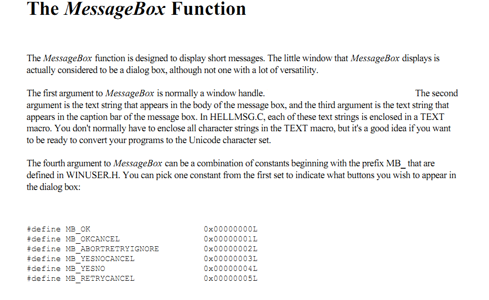
You format dates and times by selecting the cells and then using the Number Format control in
the Home➜Number group (see Figure 6-1). This control offers two date formats and one time
format.

Figure 6-1: Use the Number Format drop-down list to change the appearance of dates and times.

             When you create a formula that refers to a cell containing a date or a time, Excel may
             automatically format the formula cell as a date or a time. Sometimes, this is very help-
             ful; other times, it’s completely inappropriate and downright annoying. Unfortunately,
             you cannot turn off this automatic date formatting. You can, however, use a shortcut
             key combination to remove all number formatting from the cell and return to the
             default General format. Just select the cell and press Ctrl+Shift+~.

If none of the built-in formats meet your needs, you can create a custom number format. Select
the More Number Formats option from the Number Format drop-down list to display the Number
tab in the Format Cells dialog box. The Date and Time categories provide many additional for-
matting choices. If none of these are satisfactory, select the Custom category and type the cus-
tom format codes into the Type box. (See Appendix B for information on creating custom
number formats.)

Counting the number of words in a cell

Counting the number of words in a cell

The following formula returns the number of words in cell A1:

=LEN(TRIM(A1))-LEN(SUBSTITUTE((A1),” “,””))+1

The formula uses the TRIM function to remove excess spaces. It then uses the SUBSTITUTE func-
tion to create a new string (in memory) that has all the space characters removed. The length of
this string is subtracted from the length of the original (trimmed) string to get the number of
spaces. This value is then incremented by 1 to get the number of words.

Note that this formula returns 1 if the cell is empty. The following modification solves that problem:

=IF(LEN(A1)=0,0,LEN(TRIM(A1))-LEN(SUBSTITUTE(TRIM(A1),” “,””))+1)

             Excel has many functions that work with text, but you’re likely to run into a situation in
             which the appropriate function just doesn’t exist. In such a case, you can often create
             your own worksheet function using VBA. Chapter 25 also contains a number of custom
             text functions written in VBA.

Removing titles from names

You can use the formula that follows to remove four common titles (Mr., Dr., Ms., and Mrs.) from
a name. For example, if cell A1 contains Mr. Fred Munster, the formula would return Fred Munster.

=IF(OR(LEFT(A1,2)={“Mr”,”Dr”,”Ms”}),RIGHT(A1,LEN(A1)-(FIND(“.”,A1)+1)),A1)

Splitting text string without using formula in excel

Extracting first names, middle names, and last names

Extracting first names, middle names, and last names

Suppose you have a list consisting of people’s names in a single column. You have to separate
these names into three columns: one for the first name, one for the middle name or initial, and
one for the last name. This task is more complicated than you may initially think because not
every name in the column has a middle name or middle initial. However, you can still do it.

The formulas that follow all assume that the name appears in cell A1.
You can easily construct a formula to return the first name:
=IFERROR(LEFT(A1,FIND(“ “,A1)-1),A1)
Returning the middle name or initial is much more complicated because not all names have a
middle initial. This formula returns the middle name or initial (if it exists); otherwise, it returns
nothing:
=IF(LEN(A1)-LEN(SUBSTITUTE(A1,” “,””))>1,MID(A1,FIND(“ “,A1)+1,FIND(“ “,A1,FIND(“ “,
A1)+1)-(FIND(“ “,A1)+1)),””)
Finally, this formula returns the last name:
=IFERROR(RIGHT(A1,LEN(A1)-FIND(“*”,SUBSTITUTE(A1,” “,”*”,LEN(A1)-LEN(SUBSTITUTE
(A1,” “,””))))),””)

Extracting all but the first word of a string

Extracting all but the first word of a string

The following formula returns the contents of cell A1, except for the first word:
=RIGHT(A1,LEN(A1)-FIND(“ “,A1,1))
If cell A1 contains 2010 Operating Budget, the formula then returns Operating Budget.
This formula returns an error if the cell contains only one word. The formula below solves this
problem and returns an empty string if the cell does not contain multiple words:
=IFERROR(RIGHT(A1,LEN(A1)-FIND(“ “,A1,1)),””)
For compatibility with versions prior to Excel 2007, use this formula:
=IF(ISERR(FIND(“ “,A1)),””,RIGHT(A1,LEN(A1)-FIND(“ “,A1,1)))

Extracting the last word of a string

Extracting the last word of a string is more complicated because the FIND function only works
from left to right. Therefore, the problem rests with locating the last space character. The formula
that follows, however, solves this problem. It returns the last word of a string (all the text follow-
ing the last space character):
=RIGHT(A1,LEN(A1)-FIND(“*”,SUBSTITUTE(A1,” “,”*”,LEN(A1)-LEN(SUBSTITUTE(A1,” “,””)))))
This formula, however, has the same problem as the first formula in the preceding section: It fails
if the string does not contain at least one space character. The following modified formula uses
the IFERROR function to avoid the error value:
=IFERROR(RIGHT(A1,LEN(A1)-FIND(“*”,SUBSTITUTE(A1,” “,”*”,LEN(A1)-LEN(SUBSTITUTE
(A1,” “,””))))),A1)
For compatibility with versions prior to Excel 2007, use this formula:
=IF(ISERR(FIND(“ “,A1)),A1,RIGHT(A1,LEN(A1)-FIND(“*”,SUBSTITUTE(A1,” “,”*”,LEN(A1)-
LEN(SUBSTITUTE(A1,” “,””))))))

Extracting the first word of a string

To extract the first word of a string, a formula must locate the position of the first space charac-
ter and then use this information as an argument for the LEFT function. The following formula
does just that:
=LEFT(A1,FIND(“ “,A1)-1)
This formula returns all of the text prior to the first space in cell A1. However, the formula has a
slight problem: It returns an error if cell A1 consists of a single word. A simple modification solves
the problem by using an IFERROR function to check for the error:
=IFERROR(LEFT(A1,FIND(“ “,A1)-1),A1)
For compatibility with versions prior to Excel 2007, use this formula:
=IF(ISERR(FIND(“ “,A1)),A1,LEFT(A1,FIND(“ “,A1)-1))

Extracting a filename from a path specification

Extracting a filename from a path specification

The following formula returns the filename from a full path specification. For example, if cell A1
contains c:\files\excel\myfile.xlsx, the formula returns myfile.xlsx.
=MID(A1,FIND(“*”,SUBSTITUTE(A1,”\”,”*”,LEN(A1)-LEN(SUBSTITUTE(A1,”\”,””))))+1,LEN(A1))
This formula assumes that the system path separator is a backslash (\). It essentially returns all
the text following the last backslash character. If cell A1 doesn’t contain a backslash character,
the formula returns an error.

Determining a column letter for a column number

Determining a column letter for a column number

This next formula returns a worksheet column letter (ranging from A to XFD) for the value con-
tained in cell A1. For example, if A1 contains 29, the formula returns AC.
=LEFT(ADDRESS(1,A1,4),FIND(1,ADDRESS(1,A1,4))-1)
Note that the formula doesn’t check for a valid column number. In other words, if A1 contains a
value less than 1 or greater than 16,384, the formula then returns an error. The following modifica-
tion uses the IFERROR function to display text (Invalid Column) instead of an error value:
=IFERROR(LEFT(ADDRESS(1,A1,4),FIND(1,ADDRESS(1,A1,4))-1),”Invalid Column”)
The IFERROR function was introduced in Excel 2007. For compatibility with versions prior to
Excel 2007, use this formula:
=IF(ISERR(LEFT(ADDRESS(1,A1,4),FIND(1,ADDRESS(1,A1,4))-1)),
“Invalid Column”,LEFT(ADDRESS(1,A1,4),FIND(1,ADDRESS(1,A1,4))-1))

Removing trailing minus signs

Some accounting systems use a trailing minus sign to indicate negative values. If you import such
a report into Excel, the values with trailing minus signs are interpreted as text.
The formula that follows checks for a trailing minus sign. If found, it removes the minus sign and
returns a negative number. If cell A1 contains 198.43–, the formula returns –198.43.
=IF(RIGHT(A1,1)=”–”,LEFT(A1,LEN(A1)–1)*–1,A1)

Counting the occurrences of a substring in a cell

The formulas in the preceding section count the number of occurrences of a particular character
in a string. The following formula works with more than one character. It returns the number of
occurrences of a particular substring (contained in cell B1) within a string (contained in cell A1).
The substring can consist of any number of characters.
=(LEN(A1)-LEN(SUBSTITUTE(A1,B1,””)))/LEN(B1)
For example, if cell A1 contains the text Blonde On Blonde and B1 contains the text Blonde, the
formula returns 2.
The comparison is case sensitive, so if B1 contains the text blonde, the formula returns 0. The fol-
lowing formula is a modified version that performs a case-insensitive comparison:
=(LEN(A1)-LEN(SUBSTITUTE(UPPER(A1),UPPER(B1),””)))/LEN(B1)

Counting specific characters in a cell

This formula counts the number of Bs (uppercase only) in the string in cell A1:
=LEN(A1)-LEN(SUBSTITUTE(A1,”B”,””))
This formula uses the SUBSTITUTE function to create a new string (in memory) that has all the Bs
removed. Then the length of this string is subtracted from the length of the original string. The
result reveals the number of Bs in the original string.
The following formula is a bit more versatile. It counts the number of Bs (both upper- and lower-
case) in the string in cell A1.
=LEN(A1)-LEN(SUBSTITUTE(SUBSTITUTE(A1,”B”,””),”b”,””))

Searching and replacing within a string excel

You can use the REPLACE function in conjunction with the SEARCH function to create a new
string that replaces part of the original text string with another string. In effect, you use the
SEARCH function to find the starting location used by the REPLACE function.
For example, assume cell A1 contains the text Annual Profit Figures. The following formula
searches for the word Profit and replaces those six characters with the word Loss:

=REPLACE(A1,SEARCH(“Profit”,A1),6,”Loss”)

This next formula uses the SUBSTITUTE function to accomplish the same effect in a more effi-
cient manner:

=SUBSTITUTE(A1,”Profit”,”Loss”)

Sunday, 18 September 2011

Followers

Blog Archive